Mutual Information Neural Estimation梳理
Mutual Information Neural Estimation
原文 参考:https://ruihongqiu.github.io/posts/2020/07/mine/
背景
互信息可以衡量两个随机变量之间的相关性:
\(I(X;Z)=H(X)-H(X|Z)=H(Z)-H(Z|X)=H(X)+H(Z)-H(X,Z)\)
互信息量和KL散度的关系如下:
\(I(X;Z)=\sum_{x\in \mathcal{X}}\sum_{z\in \mathcal{Z}}p(x,z)log\frac{p(x,y)}{p(x)p(y)}=D(p(x,y)||p(x)p(y))\)
但实际计算中,特别是对于高维空间来说,其边缘熵\(H(X)\)、\(H(Z)\)和条件熵\(H(X|Z)\)难以计算。
解决方案
作者给出了两种利用梯度下降算法逼近的互信息估计,分别是The Donsker-Varadhan representation和The f-divergence representation。
The Donsker-Varadhan representation
\(D_{KL}(\mathbb{P}||\mathbb{Q})=\sup\limits_{T:\Omega \rightarrow \mathbb{R}}\mathbb{E_{\mathbb{P}}}[T]-log(\mathbb{E_{\mathbb{Q}}}[e^T])\)
其中\(\mathbb{P}\)和\(\mathbb{Q}\)是两个任意分布,\(T\)是从样本空间\(\Omega\)映射到实数\(\mathbb{R}\)的任意函数。
证明见大佬Ruihong Qiu中2.2节
The f-divergence representation
The f-divergence representation可以看做是The Donsker-Varadhan representation的弱化版本,由2.1和不等式\(\frac{x}{e}> log\mathcal{x}\)易得。
最终形式
\(I(X;Z)\geq I_{\Theta}(X,Z)=\sup\limits_{\theta\in\Theta}\mathbb{E}_{\mathbb{P}_{XZ}}[T_{\theta}]-log(\mathbb{E}_{\mathbb{P}_X\mathbb{P}_Z}[e^{T_{\mathbb{\theta}}}])\)
我们希望用一个可以利用梯度更新的神经网络模型来计算上式,则有:
\(\hat{I(X;Z)_n}=\sup\limits_{\theta\in\Theta}\mathbb{E}_{\mathbb{P}^{(n)}_{XZ}}[T_{\theta}]-log(\mathbb{E}_{\mathbb{P}^{(n)}_X\mathbb{\hat{P}}^{(n)}_Z}[e^{T_{\mathbb{\theta}}}])\)
其中\(T\)是一个神经网络;\(X\)、\(Z\)是两个样本集。得到估计的梯度为:
\(\hat{G}_B=\mathbb{E}_B[\nabla_{\theta}T_{\theta}]-\frac{\mathbb{E}_B[\nabla_{\theta}T_{\theta}e^{T_{\theta}}]}{\mathbb{E}_B[e^{T_{\theta}}]}\)
但是这种方式是有偏的。可以通过滑动平均来估计\(\mathbb{E}_B[e^{T_\theta}]\)
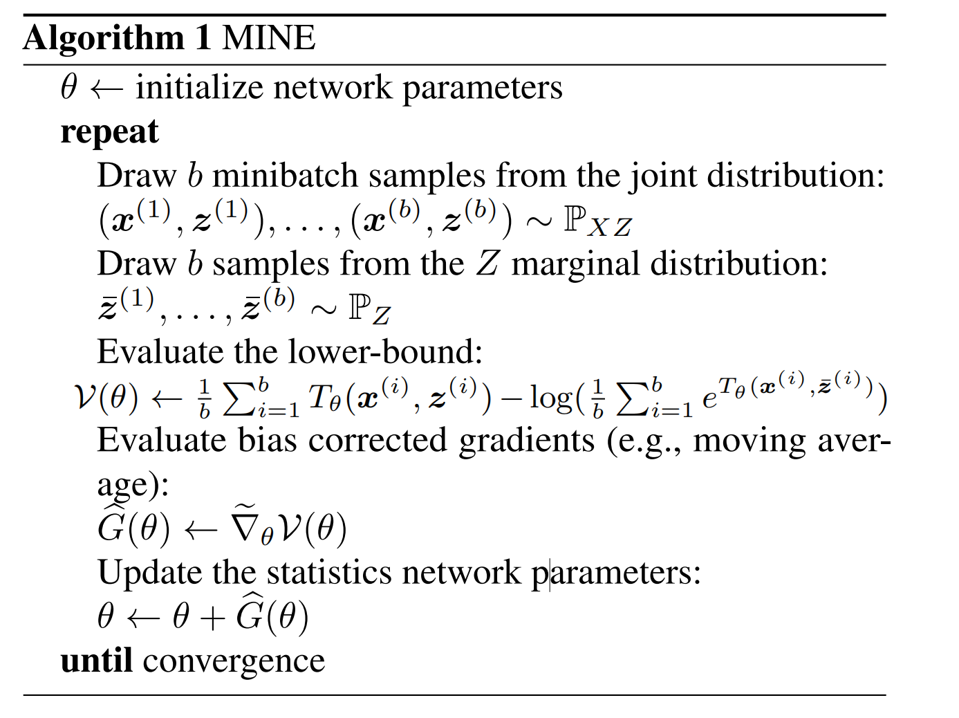
完整的过程如下: