Novel Robust Band-Limited Signal Detection Approach Using Graph梳理

Novel Robust Band-Limited Signal Detection Approach Using Graph

@TOC

Paper Download

原文百度云及提取码：9tok

Abstract

Abstract— In this letter, a novel graph-based adequate and concise information representation paradigm is explored. This new signal representation framework can provide a promising alternative for manifesting the essential structure of the communication signals. A typical application, namely, band-limited signal detection, can thus be carried out using our proposed new graph-based signal characterization. According to Monte Carlo simulation results, the proposed graph-based signal detection method leads to the outstanding performance, compared with other existing techniques especially when the signal-to-noise ratio is rather small.
Index Terms— Graph representation, cyclic spectral analysis,sparse signal, weak signal detection.

Implemention

==BY MYSELF==

一、信号的生成

根据文中叙述，使用BPSK进行作为实验数据，信噪比分别是-3dB、-7dB、-11dB、-$\infty$dB：
Matlab自带有pskmod函数:

function y = pskmod(x,M,varargin)

%PSKMOD Phase shift keying modulation
%
%   Y = PSKMOD(X,M) outputs the complex envelope of the modulation of the
%   message signal X, using the phase shift keying modulation. M is the
%   alphabet size and must be an integer power or 2. The message signal X
%   must consist of integers between 0 and M-1. For two-dimensional
%   signals, the function treats each column as 1 channel.
%
%   Y = PSKMOD(X,M,INI_PHASE) specifies the desired initial phase in
%   INI_PHASE. The default value of INI_PHASE is 0.
%
%   Y = PSKMOD(X,M,INI_PHASE,SYMBOL_ORDER) specifies how the function 
%   assigns binary words to corresponding integers. If SYMBOL_ORDER is set 
%   to 'bin' (default), then the function uses a natural binary-coded ordering. 
%   If SYMBOL_ORDER is set to 'gray', then the function uses a Gray-coded
%   ordering.
%
%   See also PSKDEMOD, MODNORM, comm.PSKModulator.

%    Copyright 1996-2013 The MathWorks, Inc.

我们可以直接调用基带调制：

MPSK=2；
msg=randi([0 MPSK-1],1,nsymbol); %生成基带数据       
msgmod=pskmod(msg,MPSK).'; %基带B-PSK调制

然后再通过载波进行搬移：

T0=1;%符号周期
fs=50/T0;%采样率
t=0:1/fs:T0-1/fs;%时间向量
fc=2/T0; %载波频率 
c=sqrt(2)*exp(1i*2*pi*fc*t);%载波信号
tx=real(msgmod*c);%载波调制

然后对所得信号进行展开，方便后续计算：

tx1=reshape(tx.',1,length(msgmod)*length(c));   %tx'的每一列是一个码元代表的采样点,现展开为一行    

现在所得信号是没有噪声的。我们通过SNR和信号功率计算噪声功率，并将信号和其对应的噪声相加，完成信号的模拟：

for indx=1:length(snr_dB)
    rx=noisegen(tx1,snr_dB(indx),T0,fs); %加入高斯白噪声后的信号
    rxy=abs(fft(rx,300));%fft
    figure(1)%显示fft图像
    subplot(4,1,indx)
    plot(rxy);
    title(['SNR=',num2str(snr_dB(indx)),'dB']);
    xlabel('fft点数','position',[320 -20]);
    ylabel('幅度');
end

其中noisegen函数是根据此PAPER自定义的噪声计算及添加。
到此完成信号生成（变换到频域）如下：
图1. 四种SNR下的BPSK信号FFT</font>

二、计算功率谱$X(m)$,并归一化

归一化公式：

$$U_X(m)= \frac{X(m)-\theta_{min}}{\theta_{man}-\theta_{man}} , m=0,1,...M-1$$

其中$X(m)$是功率谱，$\theta{max}$和$\theta{min}$是功率谱的最大值和最小值。
使用FFT计算得到功率谱$X(m)$：

$$X(m)\overset{def}{=}\frac{1}{K}|\sum_{k=0}^{K-1}x(k)e^{-j2\pi m\frac{k}{K}}|^2,0\leq m\le M-1$$

rxy=abs(fft(rx,300));%fft
Ux=zeros(1,length(rxy));
%%%%%%%%%
%Normalized
%%%%%%%%%
theta_min=min(rxy);
theta_max=max(rxy);
for m=1:1:length(rxy)
	Ux(m)=(rxy(m)- sita_min)/(sita_max-sita_min);  
end

三、量化

根据论文量化规则：

$$Q_X(m)\overset{def}{=}\triangle_\gamma(U_X(m)),m=0,1,...,M-1$$

得到量化结果：

%%%%%%%%%%%
%quantization
%%%%%%%%%%%
for mm=1:1:length(Ux)
	[~,r_level(mm)]=min(abs(Ux(mm)-r_set));%找到量化等级
end

以此步骤画图得到Fig.1

四、构建邻接矩阵、度矩阵和拉普拉斯矩阵

根据论文可总结为：

$$\widetilde{A}(Q_X(m),Q_X(m+1))=1,m=1,2,...,M-1$$

再通过线性代数定理得到Laplacian Matrix：

$$L=D-A$$

其中$L$是Laplacian，$D$ 是Degree Matrix，$A$是 Adjacency Matrix

这里用一个自己定义的函数get_LaplacianMatrix来实现：

function Lx=get_LaplacianMatrix(r,Qx)
Ax_bar=zeros(r,r);
Dx_bar=zeros(r,r);
for i =1:1:length(Qx)-1
    if(Qx(i)~=Qx(i+1))
        Ax_bar(Qx(i),Qx(i+1))=1; %半正定矩阵
        Ax_bar(Qx(i+1),Qx(i))=1; 
    end
end
for j=1:1:r
   Dx_bar(j,j)=sum(Ax_bar(j,:)); 
end
Lx=Dx_bar-Ax_bar;

五、计算Laplacian Matrix 的第二大特征值及其均值

求拉普拉斯矩阵Lx的特征值，记第二大特征值为$\lambda_1$。完成1000次计算，得到均值：

$$\bar{\lambda}_1= \frac{1}{\psi}\sum_{\nu=1}^{\psi}\lambda_1(\nu)$$

Lx=get_LaplacianMatrix(r,r_level);%得到laplacian 矩阵
[~,lamda]=eig(Lx);%计算特征值
[not_sort,~]=max(lamda);%提取特征值
lamda_sort=sort(not_sort);%特征值排序
lamda0(indx2)=lamda_sort(end-1);%找到第二大特征值

六、判断

==根据文中理论，全联通图的$\bar{\lambda}_1$应该等于量化等级$\gamma$:

${\lim_{x \to \infty}}\lambda_1=\gamma$即信噪比很小或全是白噪声时，$|\lambda_1-\gamma|<\delta$。$\delta$是一个很小门限参数。==

此处定理有待证明。。。

Question

此篇文章出了一个大BUG，通过SNR计算噪声功率出现了错误。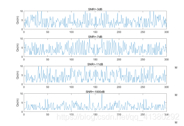

图2. 正确信噪比下的信号FFT</font>

图3. 文章中的信噪比下的信号FFT</font>

图4. 正确信噪比下逼近结果</font>

图5. 文章中信噪比下的逼近结果</font>

可见，文章中的信噪比添加方式是错误的，没有考虑白噪声的功率谱。
完整代码见My Github ==Give me a star plz!==