知识储备-矩阵相关
整理常见的矩阵理论相关知识
Hadamard product \(\to \textbf{A}\circ\textbf{B}\)
介绍
参考百度百科[1]
设\(\textbf{A},\textbf{B}\in\mathbb{C}^{m\times n}\),且\(\textbf{A}=\{a_{ij}\},\textbf{B}=\{b_{ij}\}\),则: \[ \left[\begin{array}{cccc} a_{11} b_{11} & a_{12} b_{12} & \cdots & a_{1 n} b_{1 n} \\ a_{21} b_{21} & a_{22} b_{22} & \cdots & a_{2 n} b_{2 n} \\ \vdots & \vdots &\ddots & \vdots \\ a_{m 1} b_{m 1} & a_{m 2} b_{m 2} & \cdots & a_{m n} b_{m n} \end{array}\right] \] 即对应元素相乘[1],称为矩阵\(A\)与矩阵\(B\)的哈达玛 (Hadamard) 积。记作\(\textbf{A}\circ\textbf{B}\)
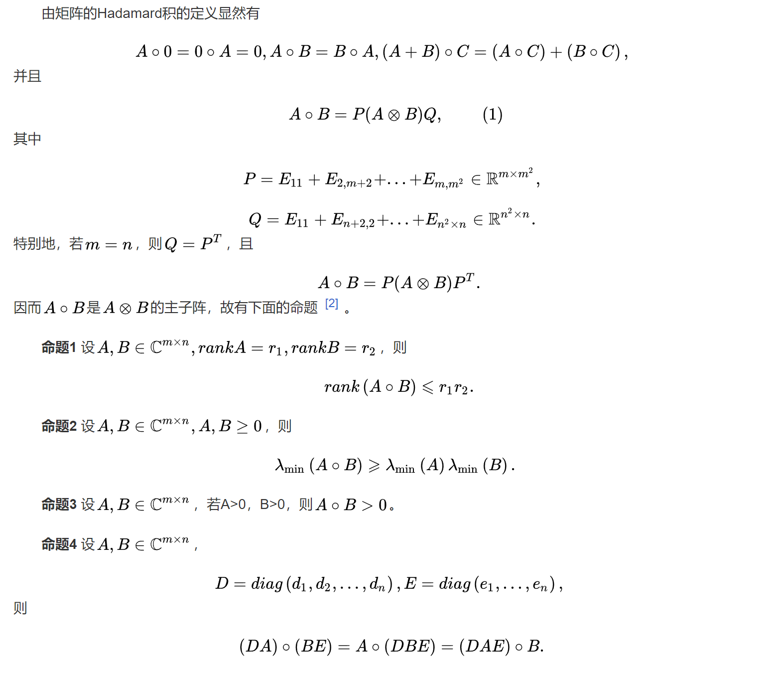
主要性质
Kronecker product \(\to \textbf{A}\otimes\textbf{B}\)
介绍
参考百度百科[2]
数学上,克罗内克积是两个任意大小的矩阵间的运算。克罗内克积是张量积的特殊形式,以德国数学家利奥波德·克罗内克命名[2]。
若\(\textbf{A}\in\mathbb{C}^{m\times n},\textbf{B}\in\mathbb{C}^{p\times q}\),则克罗内克积(Kronecker product)是一个\(\textbf{A}\otimes \textbf{B}=\textbf{C}\in\mathbb{C}^{mp\times nq}\)的分块矩阵: \[ \begin{aligned} \textbf{A}\otimes\textbf{B}=\left[ \begin{array}{ccc} a_{11}\textbf{B}&\cdots&a_{1n}\textbf{B}\\ \vdots&\ddots&\vdots\\ a_{m1}\textbf{B}&\cdots&a_{mn}\textbf{B} \end{array} \right] \end{aligned} \]
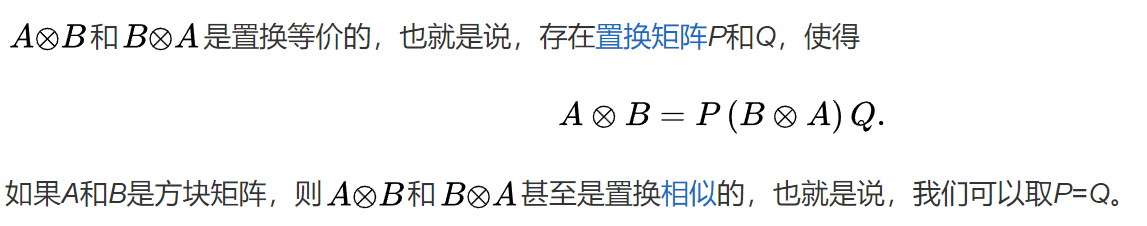
性质
满足双线性与结合律: \[ \begin{aligned} \begin{array}{c} A \otimes(B+C)=A \otimes B+A \otimes C \quad (\text{if $B$ and $C$ have the same size}) \\ (A+B) \otimes C=A \otimes C+B \otimes C \quad (\text{if $A$ and $B$ have the same size}) \\ (k A) \otimes B=A \otimes(k B)=k(A \otimes B) \\ (A \otimes B) \otimes C=A \otimes(B \otimes C) \end{array} \end{aligned} \] 不符合交换律:\(\textbf{A}\otimes\textbf{B}\)不同于\(\textbf{B}\otimes\textbf{A}\)


矩阵的迹 \(\to tr(\textbf{A})\)
介绍
参考百度百科[3]
矩阵的迹,数学、线性代数名词,在线性代数中,一个n×n矩阵\(\textbf{A}\)的主对角线(从左上方至右下方的对角线)上各个元素的总和被称为矩阵\(\textbf{A}\)的迹(或迹数),一般记作\(tr(\textbf{A})\)。[]即: \[ tr\textbf{A}=\sum\limits_{i=1}^na_{ii} \]
性质
迹是所有主对角元素的和
迹是所有特征值的和
Khatri-Rao product \(\to \textbf{A}\odot\textbf{B}\)
介绍
参考CSDN[4]
Khatri-Rao product的定义是两个具有相同列数的矩阵\(\textbf{A}\in\mathbb{C}^{I\times K},\textbf{B}\in\mathbb{C}^{J\times K}\),的对应列向量的Kronecker product排列而成的,其生成的矩阵大小为\(\textbf{A}\odot\textbf{B}=\textbf{C}\in\mathbb{C}^{IJ\times K}\)。 \[ \begin{aligned} \textbf{A}\odot\textbf{B}=\left[ \begin{array}{cccc} a_{:,1}\otimes b_{:,1}&a_{:,2}\otimes b_{:,2}&\cdots a_{:,K}\otimes b_{:,K} \end{array} \right] \end{aligned} \]
性质
\[ A \odot B \odot C=(A \odot B) \odot C=A \odot(B \odot C)\\ (A\odot B)^{T}(A \odot B)=(A^{T} A)(B^{T} B) \]
矩阵范数
矩阵1-范数(列和范数): \[ \|A\|_{1}=\max _{1 \leq j \leq n} \sum_{i=1}^{n}\left|a_{i, j}\right| \] 矩阵2-范数: \[ \|\mathrm{A}\|_{2}=\sqrt{\lambda_{\max }\left(\mathrm{A}^{\mathrm{T}} \mathrm{A}\right)} \] 矩阵F-范数: \[ \|\mathrm{A}\|_{F}=\sqrt{\operatorname{tr}\left(\mathrm{A}^{\mathrm{T}} \mathrm{A}\right)}=\sqrt{\sum_{i=1}^{m} \sum_{j=1}^{n} a_{i j}^{2}} \]
矩阵求导 Matrix Calculus
记录一下查找的矩阵求导资料,有时间再看:
标量对矩阵求导[5]
向量对矩阵求导[6]
使用科技[7]
矩阵向量化算子
矩阵向量化算子,例如文章
Compressed Channel Estimation for Intelligent Reflecting Surface-Assisted Millimeter Wave Systems. Peilan Wang et.al. IEEE Signal Processing Letters, 2020 (pdf) (Citations 72)
中出现的\(\text{vec}(\cdot)\),就是将一个矩阵的每一列首尾相连,形成一个新的列向量。 \[ \mathbf{A}\in\mathbb{C}^{m\times n}\\ \text{vec}(\mathbf{A})=[\mathbf{a}_{:m,1};\mathbf{a}_{:m,2};\cdots;\mathbf{a}_{:m,n}]\in{\mathbb{C}^{mn\times 1}} \]
Reference
- https://baike.baidu.com/item/%E5%93%88%E8%BE%BE%E7%8E%9B%E7%A7%AF/18894493?fr=aladdin ↩︎
- https://baike.baidu.com/item/%E5%85%8B%E7%BD%97%E5%86%85%E5%85%8B%E7%A7%AF/6282573?fr=aladdin ↩︎
- https://baike.baidu.com/item/%E7%9F%A9%E9%98%B5%E7%9A%84%E8%BF%B9/8889744?fr=aladdin ↩︎
- https://blog.csdn.net/xuehuitanwan123/article/details/104291475 ↩︎
- https://zhuanlan.zhihu.com/p/24709748 ↩︎
- https://zhuanlan.zhihu.com/p/24863977 ↩︎
- http://www.matrixcalculus.org/ ↩︎