mymathtools
X服从高斯分布,求\(\sin X/\cos X\)的均值高阶矩
https://zhuanlan.zhihu.com/p/515334478
\(1+\cos x+\cdots+\cos(N-1)x\)
对单独一项\(\cos nx\),乘\(\sin\frac{x}{2}\),由积化和差得: \[ \sin\frac{x}{2}\cos nx=\frac{1}{2}(\sin(\frac{x}{2})+\sin(\frac{x}{2}-nx)) \] 得求和项\(\cos x+\cos2x+\cdots+\cos(N-1)x\)为: \[ \frac{-\sin(\frac{x}{2})+\sin(\frac{x}{2}+(N-1)x)}{2\sin(\frac{x}{2})} \] 同理,\(\sin x+\sin2x+\cdots+\sin(N-1)x\)为: \[ \frac{\cos(\frac{x}{2})-\cos(\frac{x}{2}+(N-1)x)}{2\sin(\frac{x}{2})} \] matlab实现版本:
https://www.zhihu.com/zvideo/1405113965265899520
IRS计算变型
Robust Beamforming and Phase Shift Design for IRS-Enhanced Multi-User MISO Downlink Communication. Jun Wang et.al. ICC 2020 - 2020 IEEE International Conference on Communications (ICC), June 2020 (pdf) (Citations 17) \[ \begin{align} &|\mathbf{h}^\mathrm{H}\boldsymbol{\Theta}\mathbf{G}\mathbf{w}|^2\\ =&|\text{diag}(\mathbf{\Theta})^\mathrm{T}\text{diag}(\mathbf{h^\mathrm{H}})\mathbf{G}\mathbf{w}|^2 \end{align} \] 记\(\mathbf{v}=\text{diag}(\mathbf{\Theta})\),有: $$ \[\begin{align} &|\mathbf{v}^\mathrm{T}\left(\mathbf{H}+\Delta\mathbf{H}\right)\mathbf{w}|^2\\ =&\mathbf{v}^\mathrm{T}(\mathbf{H}+\Delta\mathbf{H})\mathbf{w}\mathbf{w}^\mathrm{H}(\mathbf{H}+\Delta\mathbf{H})^\mathrm{H}\mathbf{v}^\mathrm{*} \\ =&\text{vec}^\mathrm{H}(\Delta\mathbf{H})\mathbf{Q}\text{vec}(\Delta\mathbf{H})+2\Re\{\mathbf{q}^\mathrm{H}\text{vec}(\Delta\mathbf{H})\}+c \end{align}\] \[ 其中: \] =()=()^* \ =()\ c=()^() $$ 验证代码:
1 | |
还有带SINR的变型,具体可以参见:==\(\mathbf{Q}\),\(\mathbf{q}\),\(c\),==的取值会发生变化。
A Framework of Robust Transmission Design for IRS-Aided MISO Communications With Imperfect Cascaded Channels. Gui Zhou et.al. IEEE Transactions on Signal Processing, 2020 (pdf) (Citations 135)
有: \[ \mathbf{1}_M^T \mathbf{T} \overline{\mathbf{W}} \mathbf{T}^H \mathbf{1}_M=\mathbf{1}_M^T \boldsymbol{\Pi} \boldsymbol{\Xi} \boldsymbol{\Pi}^H \mathbf{1}_M \] 其中\(\mathbf{W}=\mathbf{w}\mathbf{w}^\mathrm{H}\),\(\mathbf{T}=\operatorname{diag}\left(\hat{\mathbf{g}}_{\mathbf{I} 2 \mathrm{U}}\right) \boldsymbol{\Theta} \mathbf{G}_{\mathrm{B} 2 \mathrm{I}}\),\(\boldsymbol{\Xi}=\text{diag}(\mathbf{\Theta)}\text{diag}(\mathbf{\Theta)}^\mathrm{H}\),\(\boldsymbol{\Pi}=\operatorname{diag}\left(\operatorname{diag}\left(\hat{\mathbf{g}}_{\mathrm{I} 2 \mathrm{U}}\right)\mathbf{G}_{\mathrm{B} 2 \mathrm{I}} \mathbf{w}\right)\)
验证代码:
1 | |
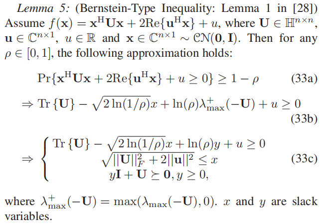
Bernstein-Type Inequality
A Framework of Robust Transmission Design for IRS-Aided MISO Communications With Imperfect Cascaded Channels. Gui Zhou et.al. IEEE Transactions on Signal Processing, 2020 (pdf) (Citations 135)
General S-Procdure
A Framework of Robust Transmission Design for IRS-Aided MISO Communications With Imperfect Cascaded Channels. Gui Zhou et.al. IEEE Transactions on Signal Processing, 2020 (pdf) (Citations 135)

moment-matching
关键词:矩匹配,PDF,CDF,逆CDF,逆累计分布函数
思想很简单,就是用Gamma分布近似一个复杂分布。由于Gamma分布的参数只与均值和方差有关,这意味着我们只要求出待求随机变量的均值和方差,就可以拟合其PDF。
1 | |
其中gaminv是Gamma分布的逆累计分布函数。alpha是 Gamma分布的shape parameter, beta是Gamma分布的scaler parameter。
AOA/AOD
关键词:LoS,视距信道,面阵,IRS
网上的对IRS面阵的空间向量的建模都是错的,这里我整理一下。
明确俯仰角/方位角
参考《现代数字信号处理及其应用》Page291 和《阵列信号处理及matlab实现》Page 42-43

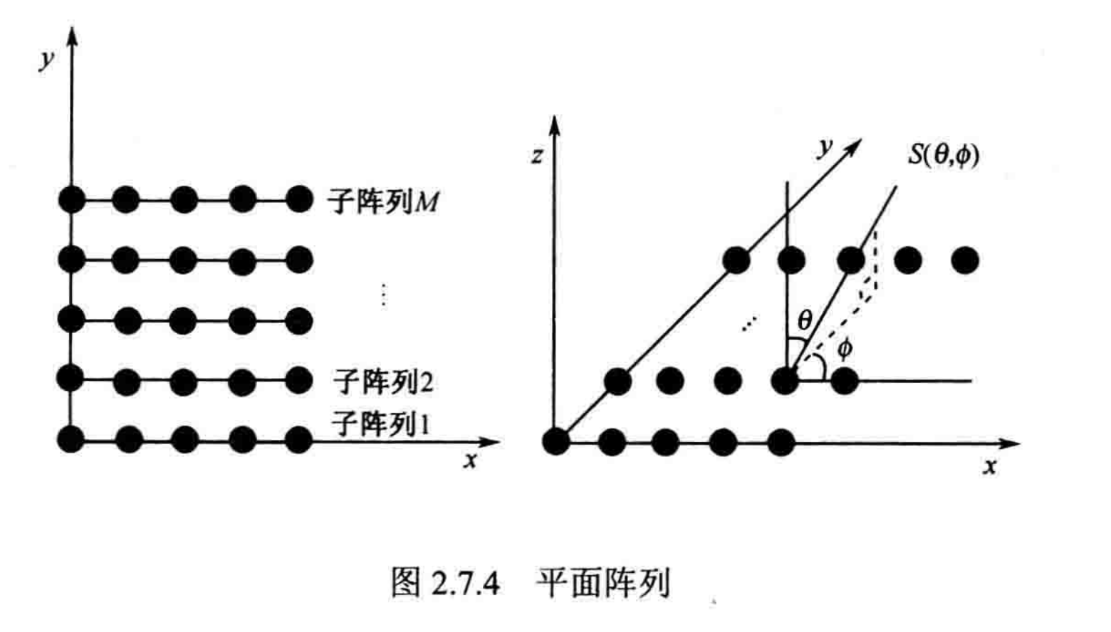
==明确以L阵的俯仰角和方位角进行建模。==
明确角度后进行分析
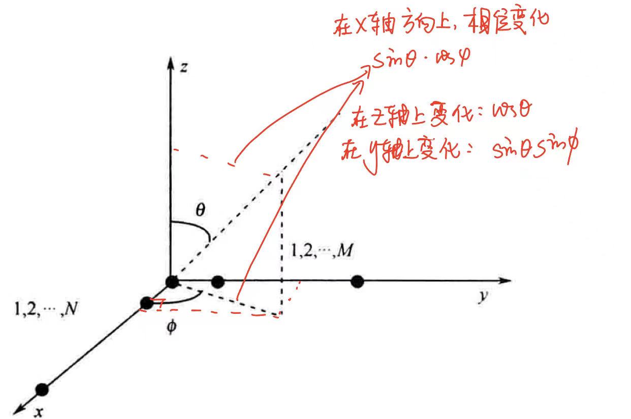
所以对于我常用的模型,
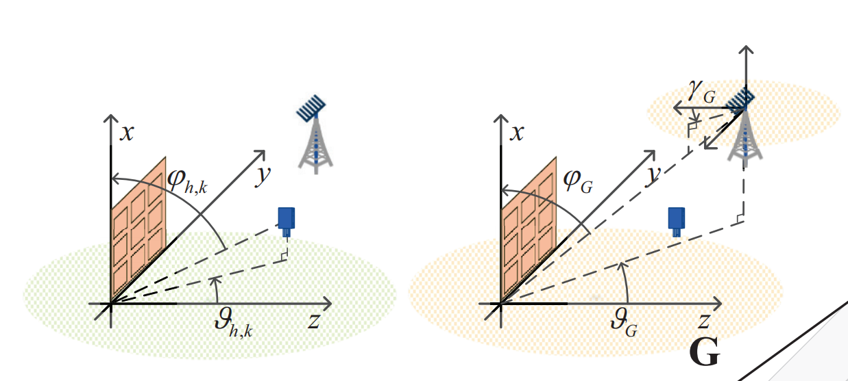
有: \[ u_{G}\triangleq 2\pi d\cos\varphi_{G} /\lambda=\pi\cos\varphi_{G}\\ v_{G}\triangleq \pi\sin\varphi_{G}\sin\vartheta_{G}\\ z_{G}\triangleq \pi\sin\gamma_{G} \]
天线的近场和远场
详细信息参见:微信公众号
主要结论 ==判断是否远场,是与天线尺寸和工作波长相关的:== \[ r\geq\frac{2d^2}{\lambda} \] 其中\(d\)为阵元之间的间隔,\(\lambda\)为波长,\(r\)为距离。